Tutorial Overview
This page provides an overview of ‘how-to’ incorporate connectivity into Marxan (Ball, Possingham, and Watts 2009), outlining instructions for using Marxan Connect, and example workflows using demographic and landscape connectivity data. These instructions assume you have already installed Marxan Connect, but if not, instructions can be found here
library(sf)

library(leaflet)

library(tmap)

library(tidyverse)

library(DT)

# set default projection for leaflet

proj <- "+proj=merc +a=6378137 +b=6378137 +lat_ts=0.0 +lon_0=0.0 +x_0=0.0 +y_0=0 +k=1.0 +units=m +nadgrids=@null +wktext  +no_defs"
1 Introduction to Marxan Connect
Marxan Connect was conceptualized in response to the growing need for connectivity to be incorporated into conservation planning on the land and sea. Our aim is to help conservation practitioners incorporate connectivity into the widely-used decision-support tool, Marxan. Marxan Connect is a graphical user interface that can be used to preprocess and prepare existing connectivity data for inclusion in a Marxan analysis (Figure 1). In terms of connectivity data, practitioners will need to have access to connectivity data (e.g. dispersal models, GPS tagging data, etc) or at least information about the landscape (see Connectivity Input section for more details). We note there are two primary ways to incorporate connectivity data into the Marxan input files: 1) as a feature, or 2) as spatial dependencies between planning units (the boundary term). The differences between these approaches are discussed in more detail below.
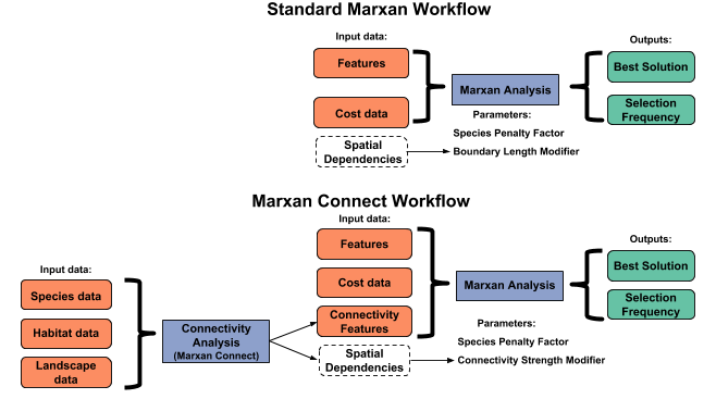
Figure 1: Comparison of workflows between the “representation only” standard approach to Marxan and “Marxan Connect.” Marxan Connect facilitates the use of connectivity data, derived from animal tagging data, genetics, dispersal models, resistance models, or geographic distance, by producing connectivity metrics and connectivity strengths (i.e. spatial dependencies that are used in the place of boundary definitions) before running Marxan. These connectivity metrics and linkage strengths are then used as inputs (connectivity-based conservation features or spatial dependencies) in the traditional Marxan workflow. The cost data in the traditional Marxan analysis refer to the cost of protecting a planning unit (i.e. opportunity cost), not the cost to traverse a landscape.
Beyond preprocessing, Marxan Connect also allows users to run the Marxan software internally or export data products (e.g. connectivity metrics, marxan files, etc) to run the analysis externally.
The Marxan Connect interface is divided into seven separate tabs, one for each step in the workflow. Below we provide a basic description of the function/s available in each step and links to several practice demonstrations.
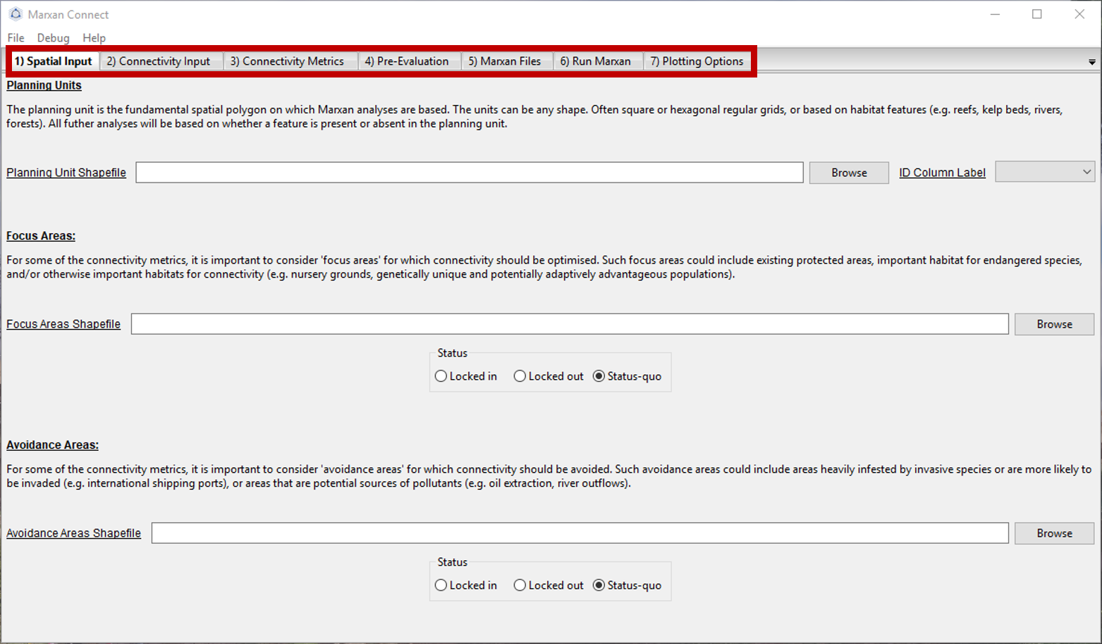
Figure 2: Tabs within Marxan Connect that represent steps in the workflow.
1.1 Spatial Input
This tab allows users to identify and load their planning units, and optionally focus areas or avoidance areas.
At this stage, Marxan Connect will choose a projection to transform all spatial data based on the geographic position and extent of the planning units. See the Projections for more details.
1.2 Connectivity Input
This tab allows users to input demographic or landscape-based connectivity data, generate landscape-based connectivity data (isolation by distance or isolation by resistance) or rescale demographic-based data. However, rescaling connectivity data can be problematic and it is recommended to collect or generate the connectivity data to the scale of the planning units.
When using a landscape connectivity approach, Marxan Connect can calculate a connectivity matrix using Euclidean distance or Least-Cost Path between the centroids of planning units or the user can import an existing landscape connectivity matrix. Other software packages such as Circuitscape (McRae, Shah, and Mohapatra 2009) and Conefor (Saura and Torné 2009) currently provide a richer set of options and specialized methods to generate custom conservation features, or connectivity matrices, both of which can then be used in Marxan Connect. For example, one could generate a network using current theory (i.e. using the movement of electrons in a circuit to approximate organism movement) using Circuitscape and input the resulting connectivity matrix into Marxan Connect to generate conservation features or spatial dependencies.
While Marxan Connect provides some tools to generate connectivity data, no single tool, tutorial or manuscript can cover this field comprehensively. Additionally, there are a number of studies and software already published on the subject (e.g. Circuitscape, LTRANS). This data can be derived from a wide variety of sources (particle tracking models, landscape models, tagging data, etc) and requires local connectivity expertise. This should be done in collaboration with local connectivity experts who already possess expertise in their specific domain.
1.3 Connectivity Metrics
This tab allows users to select which connectivity metrics to calculate and is dependent on the type of connectivity data imported on the previous tab (demographic or landscape). For example, if the user imports demographic data, only metrics under the demographic heading can be selected. At this point, users also select whether they would like to calculate metrics to create conservation features, spatial dependencies, or both.
To learn more about each of the metrics, users can select each metric from the drop down menu on the right hand side of the window to view the definition, possible objectives, equation, and an illustration to visualize how the metric works.
After selecting which metrics to calculate, users must click the “Calculate Metrics” button in the bottom right-hand corner of the window before moving onto the Pre-Evaluation tab.
1.4 Pre-Evaluation
The pre-evaluation tab allows users to modify (i.e. discretize), plot, and remove connectivity metrics calculated on the previous tab. Note than no action is required in the Pre-Evaluation tab for the spatial dependencies are calculated using the “Connectivity as boundary” option. However, if users want to include connectivity as a conservation feature, they will have to evaluate each of these metrics before moving on. Users can switch between the continuous and discretized metrics using the ‘Selection’ drop down menu.
Discretizing creates a binary spatial feature which is ‘present’ when the value of the continuous connectivity metrics is between the minimum and maximum thresholds. A summary of each metric is shown in table form on the left side of the window to help guide the user through metric modifications. The user can discretize connectivity metrics using quartiles, percentiles or custom values using the ‘Make discrete feature from minimum threshold’ and ‘Make discrete feature to maximum threshold’ panels. To view the frequency histogram for each metric, users can click the ‘Plot Frequency button beside the drop down menu for metrics. Users can also remove the selected metric if deemed not appropriate for the Marxan analysis. Once the upper and lower range of the metric are selected, users will click the ’Create New Metric’ button. This will save the modifications made to that metric and it will appear in the ‘Connectivity Metric Available for Export’ chart. Users will have to repeat this process until all desired metrics have been discretized. Note the multiple conservation features can be created from a single continuous connectivity metric.
1.5 Marxan Files
This tab allows users to append, export to ignore discrete connectivity metrics, spatial dependencies and the planning unit status to Marxan formatted files.
1.6 Run Marxan
This tab allows users to run the Marxan.exe from within Marxan Connect.
1.7 Plotting Options
This tab allows users to plot connectivity metrics and Marxan results. It also allows the users to export maps and shapefiles that contain those connectivity metrics and Marxan results.
2 Integrating connectivity data into spatial prioritization
2.1 Using connectivity data as a ‘feature’
A simple way to integrate connectivity data into spatial prioritization is to create a discrete connectivity-based conservation feature (D’Aloia et al. 2017; Magris et al. 2018; White et al. 2014). To do so requires calculating connectivity metric(s) which represent connectivity process(es) (e.g. betweenness centrality), and then choosing a threshold value(s) from the range of the metric. For example, you may wish to take only the planning units with a betweenness centrality value of 0.8 or higher, which are then converted into a discrete feature (i.e. importance areas for connectivity) (Figure 3). Under this treatment, the connectivity-based conservation feature \({j}\) in planning unit \({i}\) (i.e. \({r_{ij}}\)) becomes binary based on if the planning unit meets (1) or does not meet (0), the threshold. This type of threshold setting is often used with species distribution models, where each planning unit is assigned a probability of species occurrence, and a threshold value is used to convert these continuous distribution data to a binary map (presence vs absence or suitable vs unsuitable) for a particular species (e.g. Minor et al. 2008).
These discrete connectivity features are then treated as any other feature in Marxan, where a minimum target is set, \({T_j}\), (e.g. 50% of feature \({j}\)). In the absence of ecologically determined thresholds, an appropriate value for the thresholds and target \({T_j}\) can be determined by using a cost trade-off curve where one would test the sensitivity of the cost of the best solution and the total summed metric captured in the solution. The value of the thresholds and target \({T_j}\) could be chosen as the divergent point, where the greatest increase in the connectivity metric is achieved for a relatively small increase in cost (Figure 3) . However, the preferred approach would be to establish conservation targets which lead to a reserve network design which meets ecologically relevant conservation objective(s) such as population viability or a within network metapopulation growth rate > 1 (See “Post-hoc evaluation” section for more details).
When appropriate, high connectivity value planning units may also be “locked-in” to the ensure they are always selected in the solutions, rather than setting a target. Definitions for each connectivity based conservation feature as well as and potential conservation objectives for which they may be useful are available in Marxan Connect can be found on in the glossary.
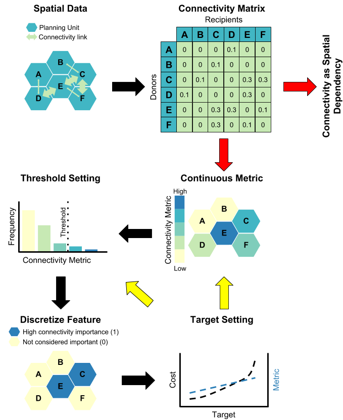
Figure 3: Data processing workflow for two possible methods for using raw connectivity data in spatial prioritization: 1) Connectivity as Spatial Dependency in the objective function (Raw Data -> Connectivity Matrix -> Connectivity as Spatial Dependency), or 1) Discrete conservation features (Raw Data -> Connectivity Matrix -> Continuous Metrics -> Threshold Setting -> Discrete Feature -> Target Setting). Black Arrows indicate a logical workflow, while red and yellow indicate a decision point. Red arrows indicate the conservation feature vs connectivity strength method decision point and yellow arrows new metric or new threshold decision point after target setting and post-hoc evaluation of conservation success.
2.2 Connectivity as spatial dependencies in the objective function
Another approach to incorporate connectivity in Marxan is using the connectivity-based data to inform the boundary cost term in the objective function (Beger et al. 2010).This cost signifies the penalty associated with protecting one site but not its well-connected partner site \({cv_{ih}}\) (Beger et al. 2010), which can be manipulated through the “Connectivity Strength Modifier” (CSM) and is similar to the BLM in standard Marxan (Figure 1). For example, as increasing the BLM reduces the edge to area ratio by minimizing costs associated with unprotected boundaries; similarly, increasing the CSM will minimize costs associated with unprotected connectivity linkages. See Beger et al. (2010); Beger et al. (2015) for examples using connectivity estimates as spatial dependencies in the objective function for MPAs in the Coral Triangle.
In Marxan Connect, one can combine the use of connectivity as spatial dependencies with a locked-in “Focus Area” (e.g. an existing protected area) to generate candidate stepping stones. However, it should be noted that the method will likely triage isolated sites out of the final solution unless these are included using other methods (e.g. a conservation feature for an isolated site which happens to contain a unique species).
3 Project Files
Marxan Connect allows users to save Marxan Connect Project files (.MarCon) which is a JSON formatted text file that stores all the filepaths, options, and connectivity metrics defined by the user. This not only allows users to start off from their last save point, but it also allows project portability and reproducibility. It is recommended to keep Marxan Connect Project files in the root directory of your project folder (i.e. the folder that contains your Marxan database) since all filepaths outside this folder will be recorded as absolute paths and then the Marxan Connect Project file will not work on another computer.
4 marxanconpy Python Module
This python module, marxanconpy, contains the mathematical heart of Marxan Connect and can be used independently via the command line.
5 Workflow Examples
We’ve provided a limited set of workflow examples designed to demonstrate some of Marxan Connect’s capabilities. These examples are for demonstration purposes and do not constitute planning advice.
Using the conservation features approach using demographic-based data
Using the spatial dependencies approach using landscape-based data
Using the spatial dependencies approach using demographic-based data (in-development)
Using the conservation features approach using landscape-based data (in-development)
References
Ball, Ian R, Hugh P Possingham, and M Watts. 2009. “Marxan and Relatives: Software for Spatial Conservation Prioritisation.” Spatial Conservation Prioritisation: Quantitative Methods and Computational Tools. Oxford University Press, Oxford, 185–95.
Beger, Maria, Simon Linke, Matt Watts, Eddie Game, Eric Treml, Ian Ball, and Hugh P Possingham. 2010. “Incorporating Asymmetric Connectivity into Spatial Decision Making for Conservation.” Conservation Letters 3 (5). Blackwell Publishing Inc: 359–68.
D’Aloia, Cassidy C, Rémi M Daigle, Isabelle M Côté, Janelle M R Curtis, Frédéric Guichard, and Marie-Josée Fortin. 2017. “A Multiple-Species Framework for Integrating Movement Processes Across Life Stages into the Design of Marine Protected Areas.” Biol. Conserv. 216 (December): 93–100.
Magris, Rafael A, Marco Andrello, Robert L Pressey, David Mouillot, Alicia Dalongeville, Martin N Jacobi, and Stéphanie Manel. 2018. “Biologically Representative and Well-Connected Marine Reserves Enhance Biodiversity Persistence in Conservation Planning.” CONSERVATION LETTERS 96 (February): e12439.
McRae, Brad H, Viral B Shah, and T K Mohapatra. 2009. “Circuitscape User Guide.” The University of California, Santa Barbara. docs.circuitscape.org.
Minor, E S, R I McDonald, E A Treml, and D L Urban. 2008. “Uncertainty in Spatially Explicit Population Models.” Biol. Conserv. 141 (4): 956–70.
Saura, Santiago, and Josep Torné. 2009. “Conefor Sensinode 2.2: A Software Package for Quantifying the Importance of Habitat Patches for Landscape Connectivity.” Environmental Modelling & Software 24 (1): 135–39.
White, J Wilson, Julianna Schroeger, Patrick T Drake, and Christopher A Edwards. 2014. “The Value of Larval Connectivity Information in the Static Optimization of Marine Reserve Design.” Conservation Letters 7 (6). Wiley Online Library: 533–44.