Connectivity as Spatial Dependency + Landscape Data
Overview
The following section provides an example of a possible workflow using landscape connectivity data as spatial dependencies (i.e. bound.dat). It is important to note that these are indeed examples of the software’s capabilities and are not intended to be used as scientific advice in a spatial conservation planning process.
The maps and plots shown in this tutorial were created in R using the shapefile exported from the “Plotting Options” tab of Marxan Connect. The R code used to make the plots can be revealed by clicking on the Code button below
library(sf)
library(leaflet)
library(tmap)
library(tidyverse)
library(DT)
# set default projection for leaflet
proj <- "+proj=merc +a=6378137 +b=6378137 +lat_ts=0.0 +lon_0=0.0 +x_0=0.0 +y_0=0 +k=1.0 +units=m +nadgrids=@null +wktext +no_defs"Case Study
In this case study, we will be working with data from the Great Barrier Reef in Australia. Our represenation features consist of a subset of bioregions identified by the Great Barrier Reef Marine Park Authority. In this example, we will generate the connectivity input data using Marxan Connect.
Input Data
Download the example project folder. This folder contains the Marxan Connect Project file, the input data, and the output data from this example.
Before opening Marxan Connect, let’s manually look through the ‘traditional’ Marxan files (spec.dat, puvspr.dat, bound.dat, and pu.dat) in the input folder of the CSD_landscape folder, which contain only representation targets. The planning unit file (hex_planning_units.shp) includes 653 hexagonal planning units that cover the Great Barrier Reef. We’ve identified a few bioregion types as our conservation features, for which we’ve set conservation targets.
spec.dat
spec <- read.csv("tutorial/CSD_landscape/input/spec.dat")
datatable(spec,rownames = FALSE, options = list(searching = FALSE))puvspr.dat
The table shown here is a trimmed version showing the first 30 rows as an example of the type of data in the puvspr.dat file. The original dataset has 974 entries.
puvspr <- read.csv("tutorial/CSD_landscape/input/puvspr.dat")
datatable(puvspr[1:30,],rownames = FALSE, options = list(searching = FALSE))bound.dat
The table shown here is a trimmed version showing the first 30 rows as an example of the type of data in the bound.dat file. The original dataset has 3600 entries.
bound <- read.csv("tutorial/CSD_landscape/input/bound.dat")
datatable(bound[1:30,],rownames = FALSE, options = list(searching = FALSE))pu.dat
The table shown here is a trimmed version showing the first 30 rows as an example of the type of data in the puvspr.dat file. The original dataset has 653 entries.
pu <- read.csv("tutorial/CSD_landscape/input/pu.dat")
datatable(pu[1:30,],rownames = FALSE, options = list(searching = FALSE))Initial Conservation Features
This map shows the bioregions, which serve as conservation features in the Marxan analysis with no connectivity.
puvspr_wide <- puvspr %>%
left_join(select(spec,"id","name"),
by=c("species"="id")) %>%
select(-species) %>%
spread(key="name",value="amount")
# planning units with output
output <- read.csv("tutorial/CSD_landscape/output/pu_no_connect.csv") %>%
mutate(geometry=st_as_sfc(geometry,"+proj=longlat +datum=WGS84"),
best_solution = as.logical(best_solution)) %>%
st_as_sf()map <- leaflet(output) %>%
addTiles()
groups <- names(select(output,-best_solution,-select_freq))[c(-1,-2)]
groups <- groups[groups!="geometry"]
for(i in groups){
z <- unlist(data.frame(output)[i])
if(is.numeric(z)){
pal <- colorBin("YlOrRd", domain = z)
}else{
pal <- colorFactor("YlOrRd", domain = z)
}
map = map %>%
addPolygons(fillColor = ~pal(z),
fillOpacity = 0.6,
weight=0.5,
color="white",
group=i,
label = as.character(z)) %>%
addLegend(pal = pal,
values = z,
title = i,
group = i,
position="bottomleft")
}
map <- map %>%
addLayersControl(overlayGroups = groups,
options = layersControlOptions(collapsed = FALSE))
for(i in groups){
map <- map %>% hideGroup(i)
}
map %>%
showGroup("BIORE_102")Adding Connectivity
The connectivity data is at the ‘heart’ of Marxan Connect’s functionality. It allows the generation of new conservation features based on connectivity metrics. Let’s examine the spatial layers we’ve added in order to incorporate connectivity into the Marxan analysis. Marxan Connect needs a shapefile for the planning units, and optionally the focus areas and avoidance areas. For simplicity, we have not included focus or avoidance areas in this tutorial. These spatial layers are shown in the map below.
# planning units
pu <- st_read("tutorial/CSD_landscape/hex_planning_units.shp") %>%
st_transform(proj)p <- qtm(pu,fill = '#7570b3')
tmap_leaflet(p) %>%
addLegend(position = "topright",
labels = c("Planning Units"),
colors = c("#7570b3"),
title = "Layers")IsolationByDistance.csv
The connectivity data for this analysis can be found in the IsolationByDistance.csv file in the CSD_landscape folder. This connectivity data was generated by Marxan Connect and represents an estimate of the proportion of those individuals originating from a donor planning unit (which contains a particular habitat type) which arrive into a recipient planning unit (which contains that same habitat type) (i.e. a probability matrix) in a edge list with type (i.e. habitat type) format. The connectivity data generating procedure is described in more detail in the Connectivity Input section. Below is the connectivity matrix of our example conservation priority. For the sake of your web browser, this table only contains the 7 rows and columns of the connectivity matrix. The real file has 1279227 entries.
conmat <- read.csv("tutorial/CSD_landscape/IsolationByDistance.csv")
datatable(conmat[1:7,],rownames = FALSE, options = list(searching = FALSE))Marxan Connect
Loading your project in Marxan Connect
Now that we have explored the input files, we are ready to open Marxan Connect and load our project. Please load the tutorial.MarCon file in the CSD_landscape folder into Marxan Connect. You should not have to change any inputs in the project, but it is important to understand what these choices entail.
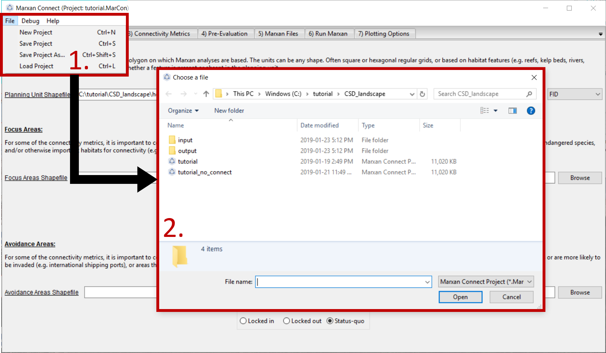
Figure 1: Loading Marxan Connect tutorial .
We will now step through the Marxan Connect workflow following the work flow tabs.
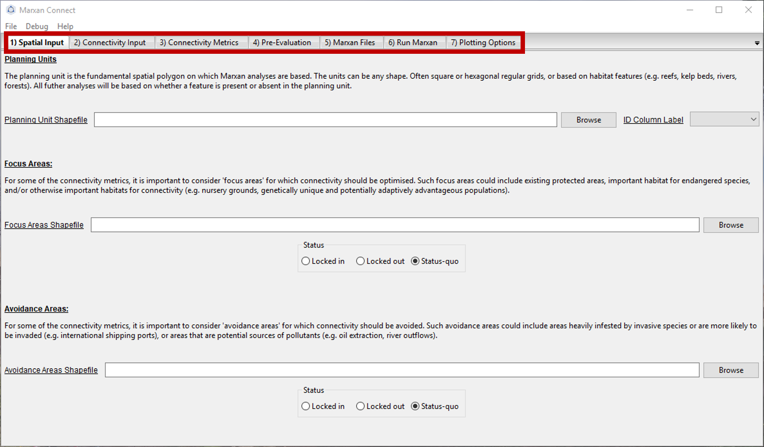
Figure 2: Workflow tabs .
Spatial Input
After loading tutorial.MarCon your Spatial Input tab should now look something like this:
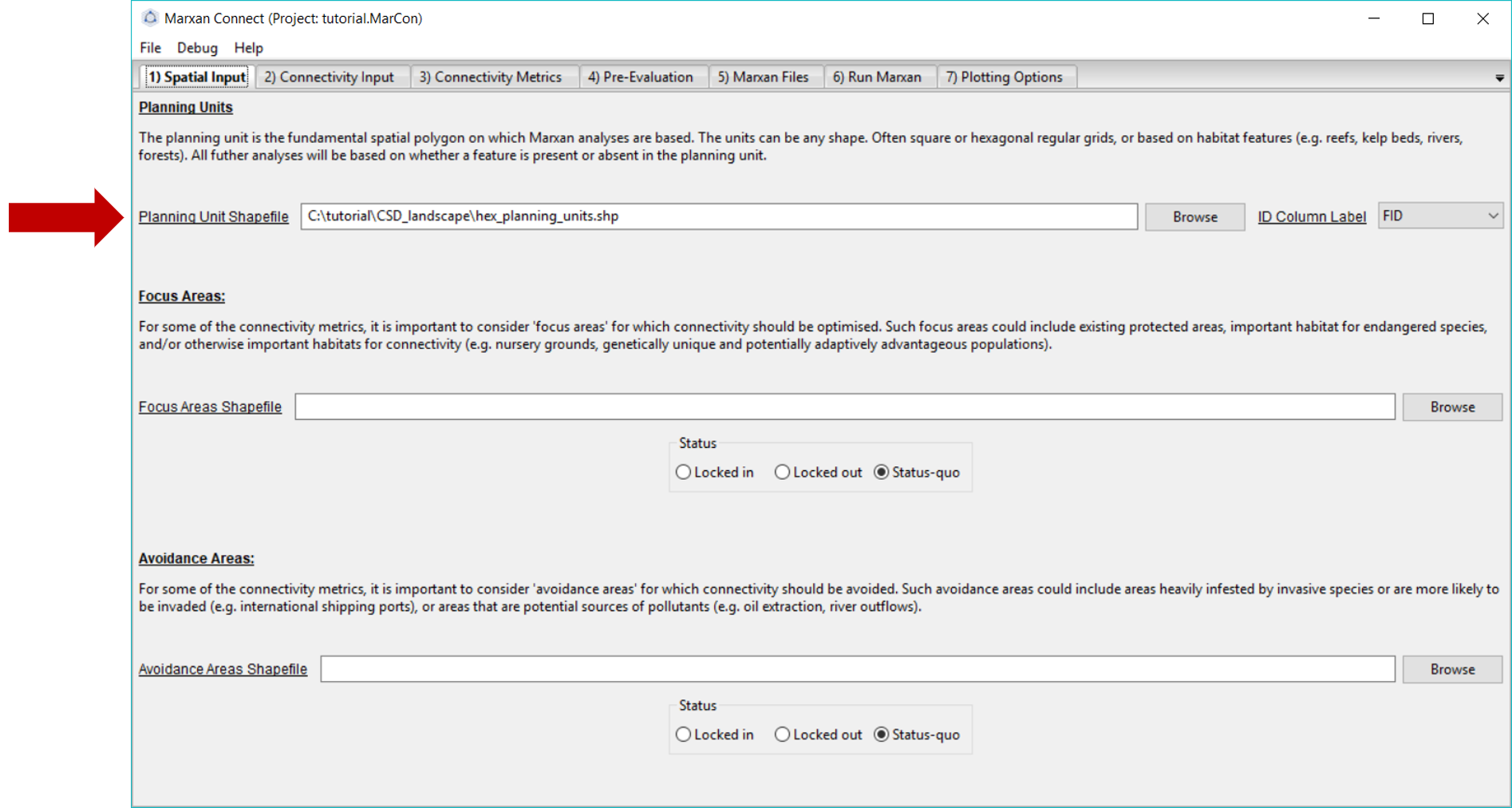
Figure 3: Spatial Input tab .
Make sure that the Planning Unit Shapefile and when relevant, the, Focus Area Shapefile and Avoidance Area Shapefile correspond to the appropriate input files (the Focus and Avoidance areas are not used in this example). On this tab, you can also choose whether the Focus Area Shapefile and Avoidance Areas Shapefile should be locked in, locked out, or status-quo (i.e. the planning unit status stays the same as what is designated in the pu.dat file).
Now we are ready to proceed to the Connectivity Input tab.
Connectivity Input
Since we are working with landscape data, we choose the Landscape Input option from the Choose Connectivity Input Category dropdown menu. Alternatively, Demographic Input could be chosen (see demographic connectivity tutorial).
For the landscape connectivity approach, Marxan Connect calculates connectivity based either habitat type and isolation, or resistance surfaces (note: latter still in development). Alternatively, users can directly provide connectivity data as a “(Edge List with Habitat)[glossary.html#edge-list-with-habitat]”. When using habitat type and isolation users can choose between Euclidean distance (i.e.) isolation by distance) or least-cost path between the centroid of planning units (i.e. isolation by resistance).
The connectivity data we use in this example was created using the “Habitat Type + Isolation” option from the second dropdown menu. We selected the “Euclidean Distance”Distance Calculation Type" to estimate the connectivity between each planning unit. We selected the bioregion_short.shp as the Habitat Type Shapefile so that pairs of planning units which contain the same habitat type are connected while others are not. The probability of connectivity then becomes \({1/distance^2}\), if pairs of planning units contain the same habitat type, and are normalized for each source planning unit so that the sum of probabilities equals 1 (i.e. row normalized). The Habitat Neighbour Buffer is the maximum distance (in meters) that neighbouring planning units could be considered directly connected. In this case, it is set to 1 meter. The Habitat Connectivity Lower Threshold is the value below which connectivity links are considered negligible and set to 0.
Since the process of creating the landscape connectivity matrix is fairly time consuming we’ve provided the pre-calculated matrix using the above options. On this tab, ensure that the Landscape Connectivity Matrix refers to the correct file. For this example, this should read IsolationByDistance.csv.
Your Connectivity Input tab should look like this (you should not have to change any settings):
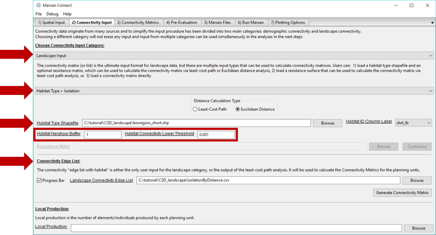
Figure 4: Connectivity Input Tab .
Now proceed to the Connectivity Metrics tab.
Connectivity Metrics
In this example, we have chosen to incorporate landscape connectivity data as the spatial dependencies between planning units, and therefore, have selected the Connectivity as boundary option in the Planning Unit Dependency as Boundary Definition section. This option uses the strengths of connectivity as the spatial dependencies (i.e. instead of the shared boundary lengths) so it can later be exported into the bound.dat file (see Beger et al. (2010) for an example). This method assumes the user has provided appropriate connectivity data (e.g. appropriate scale, units, and rank-order).
Alternatively, landscape connectivity data could be incorporated as a discrete conservation feature. The drop down menu in the top right corner gives definitions, possible objectives and the mathematical formulations for different conservation feature options. See demographic connectivity tutorial for more information.
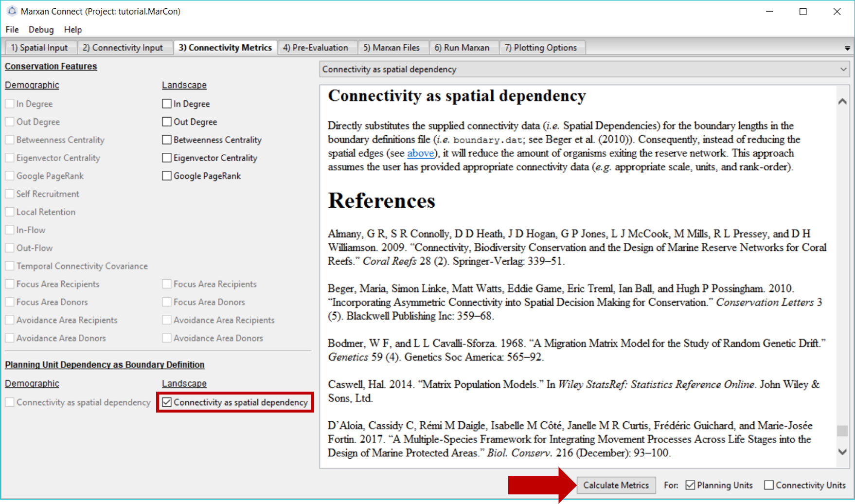
Figure 5: Connectivity Metrics Tab .
Once you have selected the appropriate landscape connectivity inputs press Calculate Metrics and proceed to the Pre-Evaluation tab. You will normally get a few warnings here. The first: “All connectivity values for type ‘N’ are below or equal to zero, excluding from futher analysis” says that the habitat type ‘N’ has no connectivity, so it will not be used in any analyses. The second: “A connectivity Edge List with Habitat was provided. The Ecological Distance to be used as the Boundary Definitions will be calculated from the mean of connectivity matrices supplied” means that you have supplied connectivity data for more than one type of habitat, so the average strength of connectivity of all (non-zero, i.e. not ‘N’) habitats will be used.
Pre-Evaluation
This page allows you to evaluate the metrics created on the Connectivity Metrics tab in more detail. It also allows you to choose how you would like to create the connectivity metrics file for further analysis. Since we are using connectivity as boundaries, we do not need to create new features. However, if you are using both spatial dependencies and conservation features, you will need to create features for those metrics. You may now proceed to the Marxan Files tab.
Marxan Files
In this example, we have not created any new conservation features, so we can ignore all file inputs/exports except the Spatial Dependencies section.
Under the Spatial Dependencies (boundary.dat) File section, we can specify the name of our new boundary file. Make sure the Original Spatial Dependencies File lists the original bound.dat file, and choose a desired name for the new bound.dat file (e.g. bound_connect.dat). If both files have the same name, the original bound.dat file will be overwritten. Once the desired options have been chosen, press Export button next to the new spatial dependencies file name. This will create a new boundary file that incorporates the landscape connectivity metrics (or update the files, as it has already been created) in the input folder of the CSD_landscape folder. A pop-up window should appear signifying that the file was exported successfully.
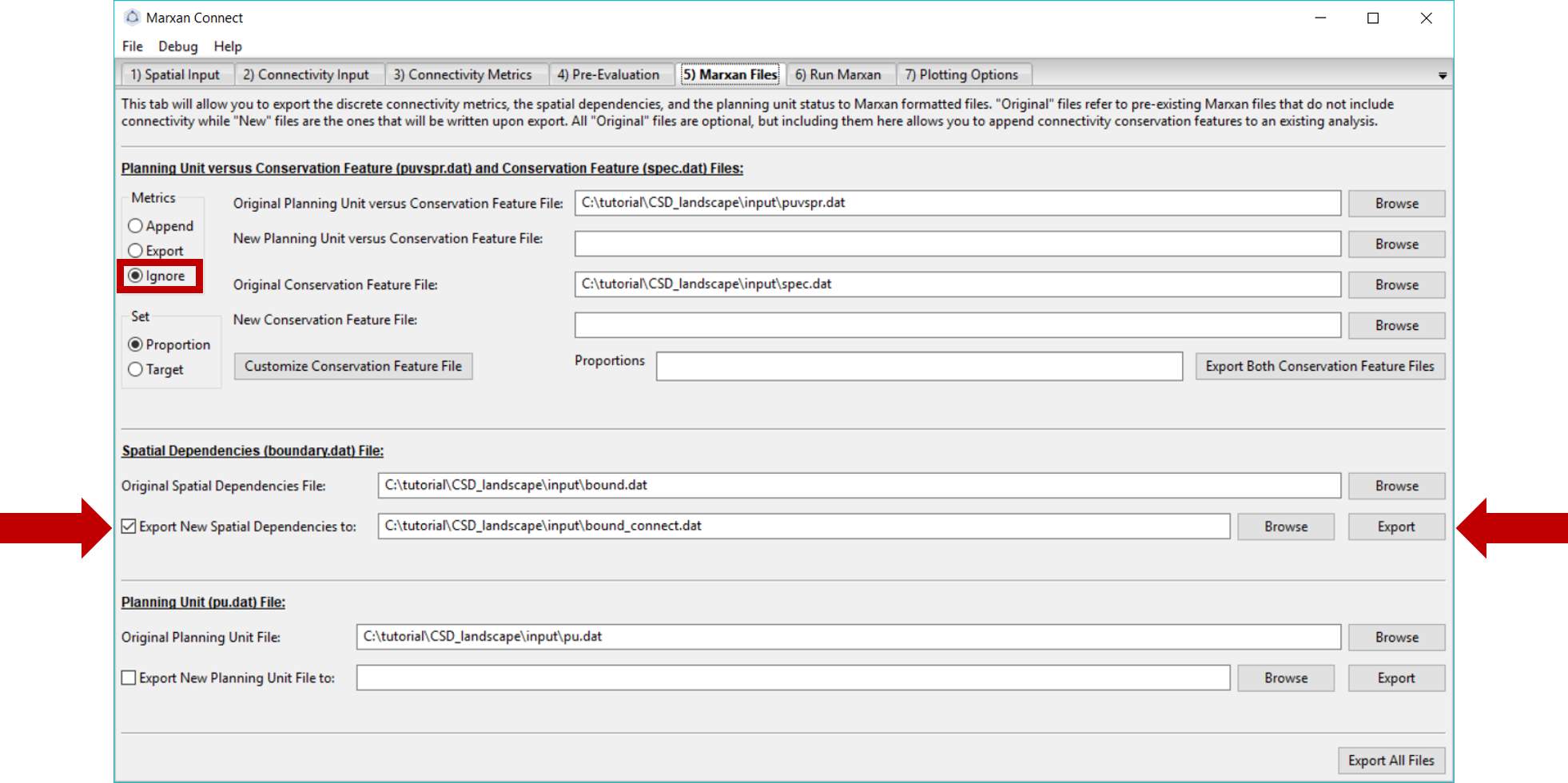
Figure 6: Marxan Files Tab .
Let’s examine the appended file.
bound_connect.dat
Locate the bound_connect.dat file that was created in your Marxan directory folder. This file should look like the table below. This table represents the spatial dependence boundaries between planning units as the values in the connectivity matrix from above (IsolationByDistance.csv, i.e. connectivity strength instead of boundary length).
The table shown here is a trimmed version showing the first 30 rows as an example of the type of data in the bound_connect.dat file. The original dataset has 38648 entries.
bound <- read.csv("tutorial/CSD_landscape/input/bound_connect.dat")
datatable(bound[1:30,],rownames = FALSE, options = list(searching = FALSE))Run Marxan
On this tab, we will run Marxan via Marxan Connect. Marxan Connect allows users to generate a Marxan input file (i.e. input.dat) from a Default template or a user defined template. Users should set their commonly used Marxan parameters (e.g. Repeat Runs, Scenario Name), choose whether to use the Original (i.e. without connectivity) or New (i.e. with connectivity) Conservation Features (i.e. puvspr.dat and spec.dat), Spatial Dependencies (i.e. bound.dat), or Planning Unit status files (i.e. pu.dat). In this example since we have only modified the spatial dependencies we will select New for those, but Original for the other files. Using spatial dependencies requires two more options Spatial Dependencies Type and the Connectivity Strength Modifier (or Boundary Length Modifier). In this case, the connectivity matrix is Symmetrical and a Connectivity Strength Modifier of 50 provided a reasonable balance between conservation outcomes and cost. To generate a new Marxan input file from the template and selected options, click on the Generate New Input File From Template. You can view or customize this file further by clicking on the Customize button. Please see the traditional Marxan documentation for more information
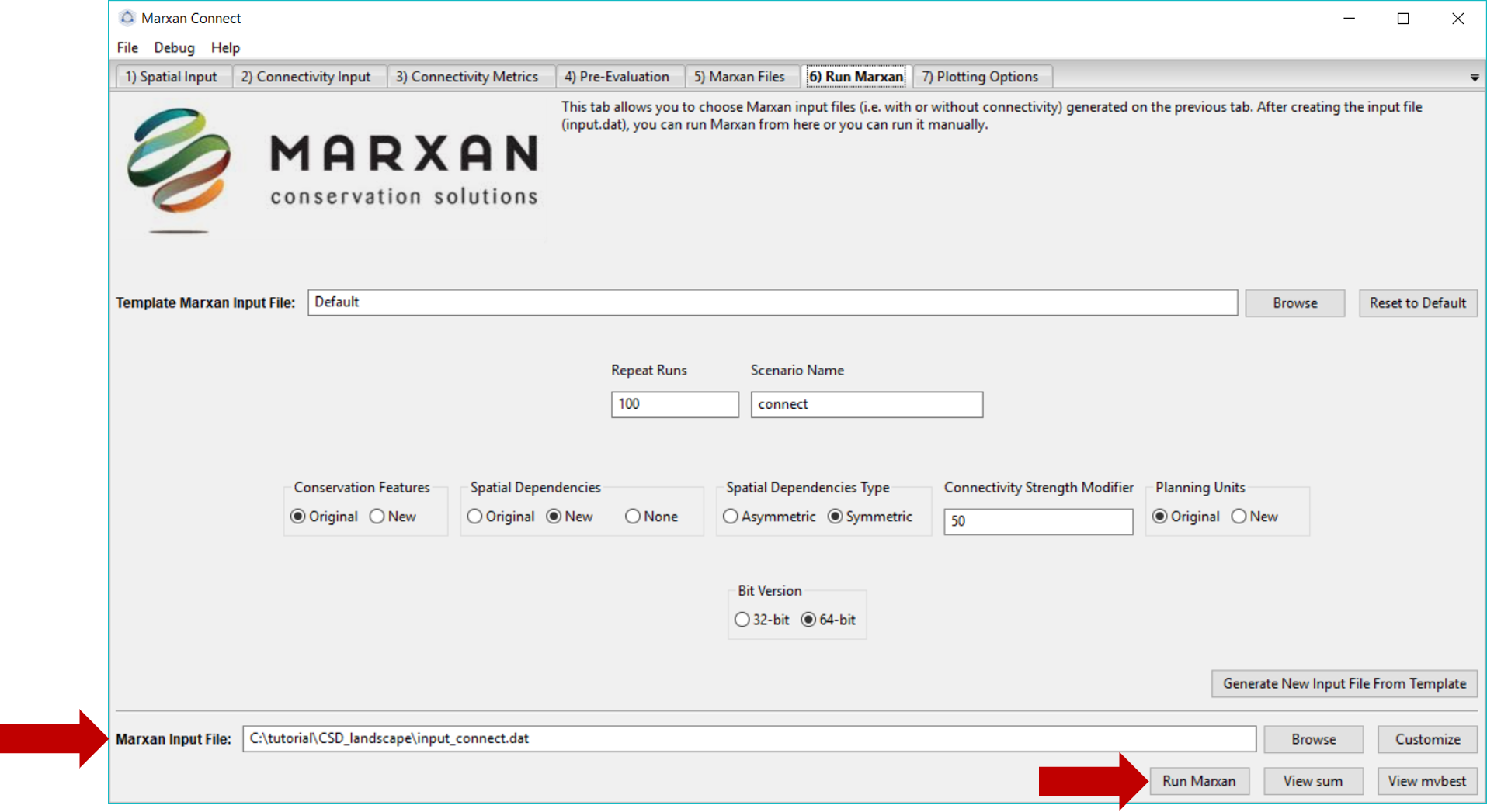
Figure 7: Marxan Analysis tab .
To run Marxan Connect press the Run Marxan button in the bottom right corner of this tab. Running Marxan with the new spatial dependencies will take much longer (~6h) since there are so many spatial dependencies. Finally, running Marxan with the connectivity conservation features and boundary definitions results in the following different Marxan solution:
# planning units with output
output <- read.csv("tutorial/CSD_landscape/output/pu_connect.csv") %>%
mutate(geometry=st_as_sfc(geometry,"+proj=longlat +datum=WGS84"),
best_solution = as.logical(best_solution)#,
# fa_included = as.logical(gsub("True",TRUE,.$fa_included)),
# aa_included = as.logical(gsub("True",TRUE,.$aa_included))
) %>%
st_as_sf()map <- leaflet(output) %>%
addTiles()
groups <- c("best_solution","select_freq")
for(i in groups){
z <- unlist(data.frame(output)[i])
if(is.numeric(z)){
pal <- colorBin("YlOrRd", domain = z)
}else{
pal <- colorFactor("YlOrRd", domain = z)
}
map = map %>%
addPolygons(fillColor = ~pal(z),
fillOpacity = 0.6,
weight=0.5,
color="white",
group=i,
label = as.character(z)) %>%
addLegend(pal = pal,
values = z,
title = i,
group = i,
position="bottomleft")
}
map <- map %>%
addLayersControl(overlayGroups = groups,
options = layersControlOptions(collapsed = FALSE))
for(i in groups){
map <- map %>% hideGroup(i)
}
map %>%
showGroup("select_freq")Here is the output of our example with no connectivity for comparison.
# planning units with output
output <- read.csv("tutorial/CSD_landscape/output/pu_no_connect.csv") %>%
mutate(geometry=st_as_sfc(geometry,"+proj=longlat +datum=WGS84"),
best_solution = as.logical(best_solution)) %>%
st_as_sf()map <- leaflet(output) %>%
addTiles()
groups <- c("best_solution","select_freq")
for(i in groups){
z <- unlist(data.frame(output)[i])
if(is.numeric(z)){
pal <- colorBin("YlOrRd", domain = z)
}else{
pal <- colorFactor("YlOrRd", domain = z)
}
map = map %>%
addPolygons(fillColor = ~pal(z),
fillOpacity = 0.6,
weight=0.5,
color="white",
group=i,
label = as.character(z)) %>%
addLegend(pal = pal,
values = z,
title = i,
group = i,
position="bottomleft")
}
map <- map %>%
addLayersControl(overlayGroups = groups,
options = layersControlOptions(collapsed = FALSE))
for(i in groups){
map <- map %>% hideGroup(i)
}
map %>%
showGroup("select_freq")Plotting Options
Here the users can plot up to two layers of input or output data on a built in basemap (provided by the basemap package). The tab allows users to choose a few basic color, transparency, and legend positioning options, but this tab also allows users to export the output data in various formats to provide further plotting or analysis options.